How to Trade Options: Interest Rates, Dividends, Calls Versus Puts
Volatility, Movement, Interest Rates, Dividends, Option prices
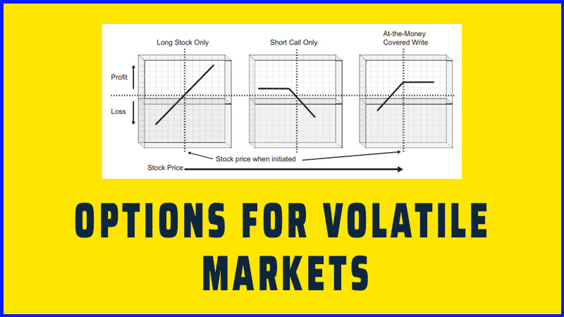
Course: [ OPTIONS FOR VOLATILE MARKETS : Chapter 2: Option Pricing and Valuation ]
Options |
Volatility is a measure of how much a security has previously moved in a given amount of time either up or down, and by implication, a measure of the future potential movement.
Volatility
Volatility is a measure of how much a
security has previously moved in a given amount of time either up or down, and
by implication, a measure of the future potential movement. It is important in
determining an option’s theoretical value, and it is essentially the factor in
the formula that accounts for the probability that the underlying stock can
move to or beyond the strike price before the expiration date. If a high-beta
(highly volatile) semiconductor stock and a conservative bank stock are both
trading at $30 a share, you would not expect both to have the same probability
of reaching $35 by a certain date. Their option prices would reflect this
difference as a consequence of their different volatilities.
Historical volatility is calculated
using the statistical formula for the standard deviation of a previous set of
prices over a defined time period—typically 20, 50, or 100 days. One problem
with that, however, is that each of these time periods can yield a slightly
different volatility value and different data sources use different sets of
historical values for their calculation. The greater issue is that none of the
historical probability periods may produce an accurate prediction of the
stock’s future volatility. The market may therefore price an option quite
differently from its theoretical price. It is important to know all this so
that you can keep a realistic perspective on the theoretical prices you see for
options on quote screens or other services.
As discussed in the Introduction, it is
really the implied volatility of an option (that which is determined in the
marketplace) rather than the historical volatility (calculated from historical
data) that is key, since what you pay for an option is determined by the
implied volatility. But it is the historical volatility that is used to create
the theoretical value that we at least use as a rough benchmark to determine
whether an option is undervalued, fairly valued, or overvalued.
Volatility is discussed in greater
detail in Chapter 9.
Interest Rates
Interest rates play a role in
determining option prices as they affect the cost an arbitrageur would have to
pay to carry a riskless stock-and-option position. Although a very minor one
from day to day, the effect can be noticeable when comparing option prices
during periods of very low interest rates with those of very high interest
rates. For the short duration of most option trades, the impact of interest
rates will be imperceptible unless they are changing somewhat dramatically in a
short period of time—say, weeks. Option writers can expect to get slightly
higher option premiums when interest rates are higher, all other things being equal.
Dividends
Option prices are affected by
dividends, although some models omit them for convenience. Since dividends are
cash distributions to shareholders from the earnings of the company, once paid,
they are no longer part of the company’s net worth. To reflect this fact, the
stock price is reduced on the appropriate date by the amount of the dividend
(and the stock is therefore said to trade ex-dividend on that date). No
adjustments are made to the price or terms of options on stocks that pay dividends.
Therefore, one would expect call options to be priced somewhat lower for stocks
paying dividends and put prices somewhat higher, since the option buyer gets no
benefit from the payout. Furthermore, the dividend represents value that is
removed from the company’s net worth each quarter rather than being reinvested
inside the company and thus reduces the growth prospects of the stock. Indeed,
the value of a call option does tend to be lower on a dividend stock and put
options slightly higher because buyers know the stock price will be lowered on
the ex-dividend date. As the dividend approaches, options tend to anticipate
the expected drop in value caused by the dividend.
The change is very slight and occurs
gradually, and because the stock price is continually changing, there is no
arbitrage that can take advantage of this option price change on a riskless
basis. There is, however, a common arbitrage on dividend paying stocks whereby
arbs will buy the stock, sell ITM call options that expire after the dividend
will be paid, and purchase puts at the same strike price and month. The
position is placed at a net price equal to the strike price (give or take a few
cents) such that if arbs are assigned on the stock prior to the dividend, they
make no money. But they don’t lose any either, and if they are not assigned,
they pocket the dividend and then exercise their put to sell the stock, earning
a dividend payment that was acquired with virtually no risk. Dividend arbitrage
on certain stocks can occur on millions of shares. As such, investors
implementing option strategies on high dividend-paying stocks should be aware
of this arb activity.
Calls versus Puts
Our discussion thus far about option
pricing has made no real distinction between the pricing of puts and the
pricing of calls. There are, however, differences, and, while small, they are
worthy of note.
Theoretically, the price of a call
option considers the possibility of the underlying stock rising to infinity.
The put, however, accounts only for the probability that the stock goes to
zero. Stated another way, a $40 stock can only drop by a maximum of $40 or 100
percent, yet it could conceivably go up by $60 (150 percent) or more. The
probabilities of the stock going to either of these extremes during the option’s
life may be miniscule, but from a statistical perspective, they are meaningful.
They require that options pricing formulae use an assumed distribution other
than a normal (bell-shaped) distribution for prices of the underlying. The
options pricing formula developed by Fischer Black and Myron Scholes accounts
for this phenomenon by utilizing a lognormal distribution, which essentially
holds that prices may range between zero and infinity, corresponding well with
the reality of stock prices. The result is that call prices contain a small
positive bias in price over the equivalent (same strike and month) put. That is
to say, that for a stock at exactly $50 with a volatility of 20 percent, a
50-strike call with 60 days to go would theoretically be $1.64, while the
50-strike put would theoretically be $1.60.
Option Skews and Anomalies
As you will discover, some options may
trade near their theoretical values while others may deviate significantly from
the formula-derived price. You will also observe, however, that when an option
trades above or below its theoretical value, most others in the same month will
also, and by a similar amount. Both of these observations are very important to
the development of option strategies.
When demand for a specific option on a
given stock is particularly high, the price of that option will be expected to
rise, perhaps well above the theoretical value. Let’s say that XYZ is trading
at $25 and there is abnormally strong demand for the May 30 call option. As
that occurs, it presents opportunities for riskless arbitrage between that
option and its underlying stock, which tends to bring that option back into
line with other options in the same month and with the stock itself. Such
arbitrage is rather straightforward and widely practiced by professional
traders, market makers, and brokerage firms.
Aiding in the maintenance of price
relationships between options is the fact that market makers price them by
computer, and when they want to change the prices on a particular stock’s
options, they commonly do so by simply changing the implied volatility in their
pricing model. That results in all of the options on a given stock (at least
those in the same month) being ratcheted up or down, essentially in unison, by
the press of a button.
But there are other pricing anomalies
that commonly occur with option prices that cannot be rectified by an arbitrage
trade. The most common deviation in option pricing is the tendency of a given
class of options (those on the same underlying stock) to trade at prices that
imply a higher or lower volatility than the historical volatility used in the
Black-Scholes formula. This happens extremely often and is readily visible when
viewing an option chain, as both actual and theoretical prices are typically
available in most option chains. An example is illustrated in Table 2.4, using Apple Computer (AAPL).
TABLE 2.4 Market Price versus
Theoretical Value
|
Stock = AAPL Price = 348.48 (1/14/11) Option Strike = 350 Calls |
|||
|
Month |
Market Price |
Theoretical Price |
Implied Volatility |
|
Jan |
6.55 |
2.70 |
.35 |
|
Feb |
11.10 |
6.51 |
.27 |
|
Mar |
14.95 |
8.93 |
.27 |
|
Apr |
18.65 |
10.87 |
.28 |
|
Jul |
27.65 |
15.69 |
.29 |
|
Oct |
36.15 |
19.67 |
.30 |
|
Jan LEAP |
43.17 |
22.79 |
.31 |
Data source: Power Options®
www.poweropt.com/.
Table 2.4 shows us that on this day in January 2011, the market
prices of options on AAPL closed considerably higher than those calculated by
Black- Scholes. This is supported by data from McMillan Analysis Corp., showing
the actual historical volatilities for AAPL to be as follows:
|
Historical |
Volatility |
|
20-day |
11 |
|
50-day |
17 |
|
100-day |
19 |
Depending on which time period you use
for your volatility calculation, the implied volatility is almost double and,
accordingly, so are actual prices. This may be a relatively extreme example,
but the phenomenon is quite common. You will also notice that the implied
volatilities in different months are not even the same. They are very high for
the current month option, then dip by 25 percent in the next month and begin
rising each subsequent month. (The full option chain shows almost identical
implied volatilities in all strikes of the same month.) These are the realities
of option pricing.
The reasons for such a differential
between actual and theoretical pricing may be varied. The market may simply be
expecting higher volatility in future months than during the period on which
historical volatility was calculated. Or the market may be injecting a bias to
either the upside or downside on the stock, which manifests itself as a higher
implied volatility for both put and call options.
It is important to note that,
regardless of the direction of an inherent bias being priced in by the market,
both puts and calls on the same underlying will rise or fall accordingly. This
phenomenon can be very misleading to those trying to interpret a directional
message from the price of an option alone. When bad news comes out or is
anticipated on a particular stock, there may, for example, be an increased
demand for puts on that stock, causing put prices to rise above theoretical
value. What happens, due to market forces and arbitrage, is that both the puts
and calls on that stock will rise above theoretical value, and they will do so
by a similar amount (i.e., the implied volatility of the puts will be similar
to that of the calls).
Such differences in option prices between actual and theoretical or between actuals in different months are called skews—anomalies between the prices of different options on the same instrument. They cannot be arbitraged away, but they can be used in the development of option strategies that may offer a statistical advantage over time. The overvaluation in AAPL call options is somewhat akin to finding a blackjack table that pays 3-1 for a blackjack instead of 2-1. Over a large number of hands, it represents a definite statistical advantage to the player, but you still may not get one in the short run.
OPTIONS FOR VOLATILE MARKETS : Chapter 2: Option Pricing and Valuation : Tag: Options : Volatility, Movement, Interest Rates, Dividends, Option prices - How to Trade Options: Interest Rates, Dividends, Calls Versus Puts
Options |