Average True Range(ATR) Calculation: How its Work

Average True Range(ATR) Calculation

Introduction

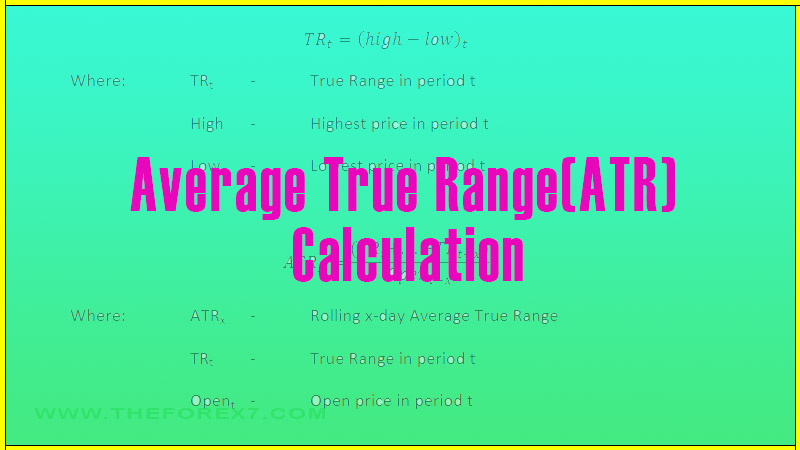
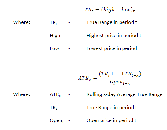
The Average True Range (ATR) of an asset is a historical volatility indicator that calculates the average of a number of previous True Range values. 

True Range (TR) of an asset can be defined as follows

The ATR and TR values allow us to understand historical volatilities, and when we compare these values across various periods we can gauge how the volatility of an asset has changed with time. By understanding ATR as a historical volatility indicator we can use it to appreciate the trading opportunities inherent in the asset and the risk that come with it.

In this example, we calculate rolling one-day ATRs for the S&P500 and compare averages of the these rolling ATRs over different periods in time.

Step One–Obtaining the Data

To begin with, we need to download an S&P500 data set:

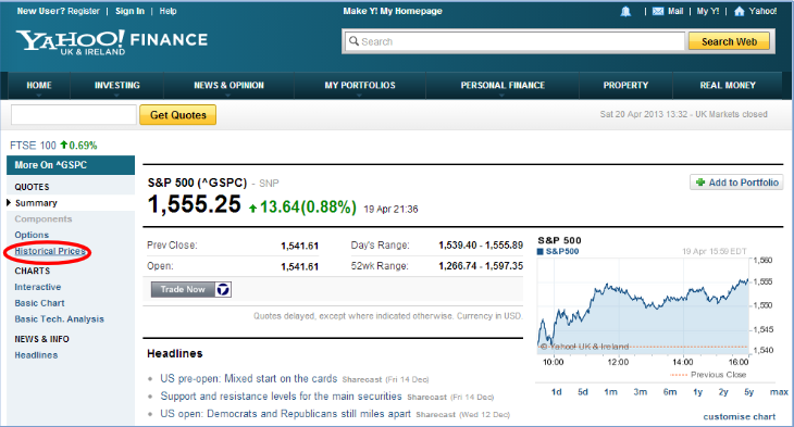
·Go to www.finance.yahoo.com

·In the quote box, type S&P and select the S&P500 from the drop-down list (ticker ^GSPC).

This will direct you to the summary page for the S&P500.

·Now navigate to the historical prices page by clicking on “historical prices” on the left-hand side.

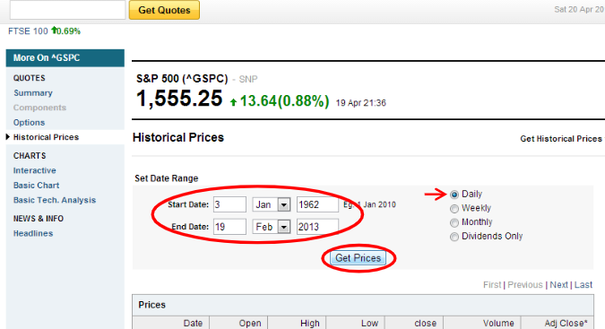
On the historical prices page, we can input the timeframe in which we want to extract prices, as well as the frequency. In this example, we will use daily data from the 3rdof January 1962 to the 19thof February 2013.

·Change the start date to “3 Jan 1962”.

·Change the end date to “19 Feb 2013”.

·Select “daily” as the frequency.

·Click “Get Prices” to update the data table.

·With the prices table updated, scroll down to the bottom of the page and click “download to spreadsheet”

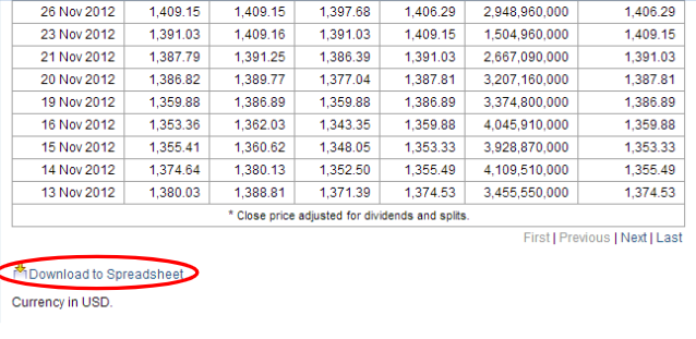
Clicking “open spreadsheet”, will open the data in Excel straight away. You then need to save the excel sheet to a folder on your hard drive to permanently store it. Alternatively, you can save the file straight to a location on your hard drive, and navigate to the file yourself and open it. Be sure to save the file after any work or edits are carried out.

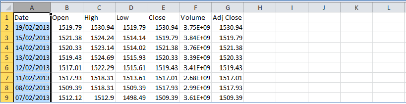
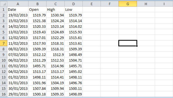
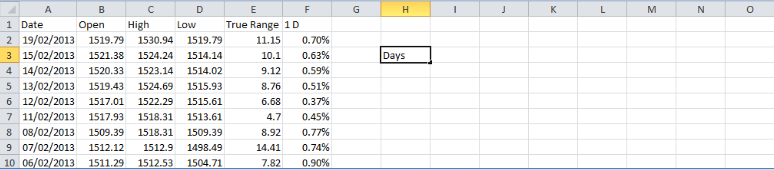
Step Two–Arranging the Data. The screenshot below shows what the excel spreadsheet should look like when opened: If the “Date” column is filled with # symbols as in the screenshot, the column width needs to be adjusted so we can see the values in full.

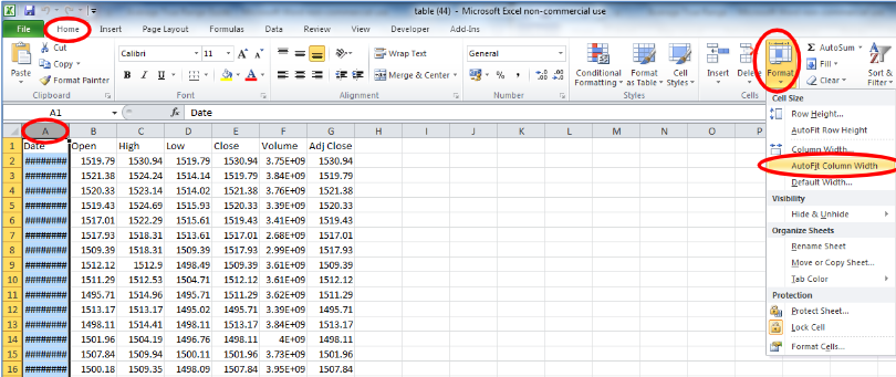
·Click on column A and navigate to Homeà For matà AutoFit Column Width.

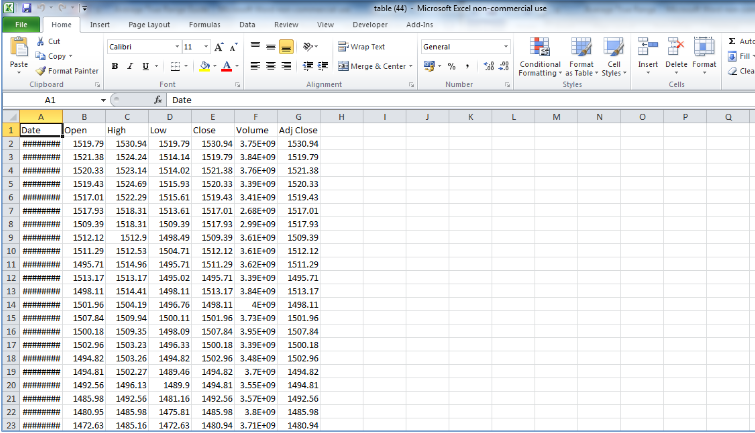
If the “Date” column is filled with # symbols as in the screenshot, the column width needs to be adjusted so we can see the values in full.

·Click on column A and navigate to Home Format Auto Fit Column Width

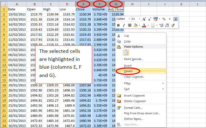
For Average True Range analysis, we only need data for the High, Low and Open prices of each day. To delete the other columns of data take the following steps:

·Click on column E.

·Hold CTRL and click on columns F and G to add these to your selection.

·Right-click on the selected area and select delete.

If you haven’t saved the spreadsheet already, save it now:

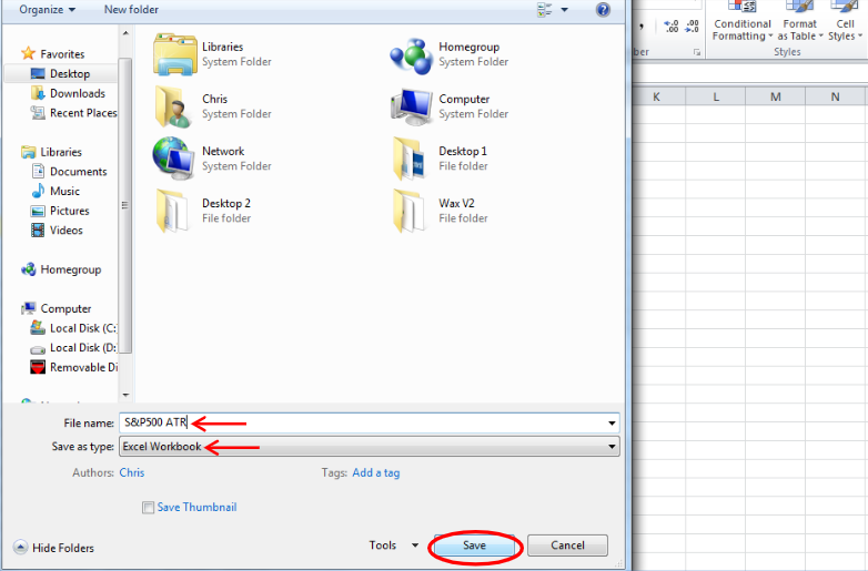
·Navigate to File Save As

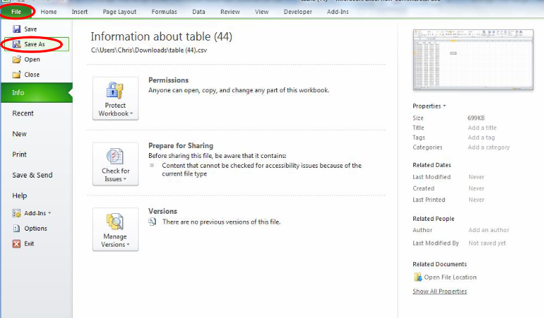
·Rename the file “S&P500 ATR” as an Excel Workbook, and save it to a preferred directory on your computer.

Step Three–Calculating the True Range and Average True Range

In this step, we will create two columns with TR and ATR data respectively. The ATR will be calculated on a rolling one-day basis.

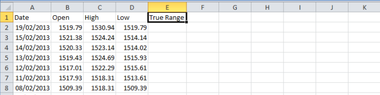
We will begin with the True Range column

·Select cell E1 and type “True Range” to head the column.

·Press Enter.

·Auto-adjust the column width as shown previously in this guide OR manually adjust the column width by clicking and dragging the intersection of columns E and F.

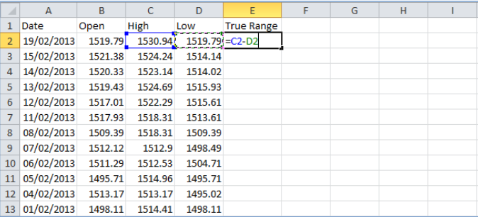
The next stage involves calculating the true range using the formula provided at the start of this guide. The True Range will simply be the High minus the Low of each day.

·Select cell E2 and type “=C2-D2”. An alternative way to enter the formula would be using the mouse to click on the desired cells (C2 and D2) at the appropriate place within the formula.

·Press Enter.

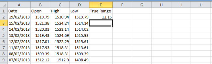
Next, we copy down the formula we just applied to cell E2, down to E12871 (the earliest date in our dataset), which saves having to type the formula into every single one of these cells.

·Navigate to the bottom of the spreadsheet by selecting a cell in columns A, B, C or D and pressing CTRL+DOWN on the keyboard.

·Next, move across to cell E12871 and press CTRL+SHIFT+UP to select all the cells from E2 to E12871

.·With the cells still selected, press CTRL+D to copy the formula down from cell E2 to all our selected cells.

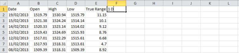
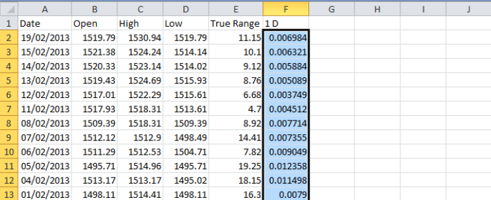
Now we have calculated the TR of each of our trading days, we move on to calculating the rolling one-day ATR at each period (day):

·Select cell F1and type “1 D”, heading a column that will contain our one-day rolling ATR. 

·Press Enter. 

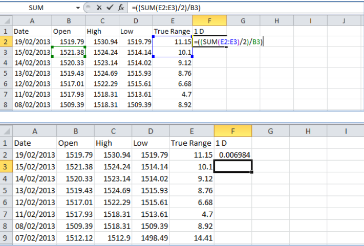
We now apply the ATR calculation as shown at the beginning of this guide.

·Select cell F2 and type “((Sum(E2:E3)/2)/B3”. Press Enter.

We are now going to copy this formula down to the entire F column –similarly to the process, we went through for calculating the TR column.

·Navigate to the bottom of the spreadsheet by selecting a cell in columns A, B, C, D or E and pressing CTRL+DOWN on the keyboard.

·Next, move across to cell F12871 and press CTRL+SHIFT+UP to select all the cells from F2 to F12871.

·With the cells still selected, press CTRL+D to copy the formula down from cell F2 to all our selected cells.

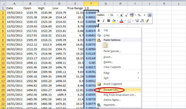
·With these cells still selected, right-click within the selection and go to “Format Cells”.

·Change the number category to display itself in percentage format with 2 decimal places. Press OK.

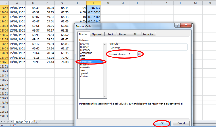
This changes all the ATR values we have just calculated to display themselves in terms of percentages. Notice how cell F12871 has an error “#DIV/0!”. This is because the ATR calculation within this cell relies on data from the previous trading day, which we do not have. Before we proceed, delete the contents of this cell.

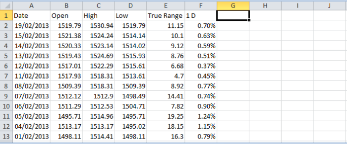
Our ATR values show an average of two day trading ranges expressed as a percentage. This allows us to track changes in the one-day ATR on a rolling basis through the historical period analyzed. To see how the one-day ATR of the S&P500 has evolved over time, we are now going to find some averages of these rolling one-day ATRs over various time horizons.

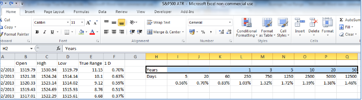
·Select cell H3 and type “Days”. Press Enter.

·In cell I3 type “5”.Press Enter.

·In cell J3 type “20”.Press Enter.

·In cell K3 type “60”.Press Enter.

·In cell L3 type “250”.Press Enter.

·In cell M3 type “750”.Press Enter.

·In cell N3 type “1250”.Press Enter.

·In cell O3 type “2500”.Press Enter.

·In cell P3 type “5000”.Press Enter.

·In cell Q3 type “12500”.Press Enter.

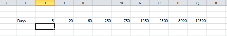
These cells represent the time horizons, expressed in days, over which we will analyze the average one-day rolling ATRs.

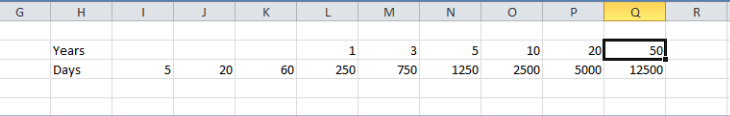
·In cell H2 type “Years”.Press Enter.

·In cell L2 type “1”.Press Enter.

·In cell M2 type “3”.Press Enter.

·In cell N2 type “5”.Press Enter.

·In cell O2 type “10”.Press Enter.

·In cell P2 type “20”.Press Enter.

·In cell Q2 type “50”.Press Enter.

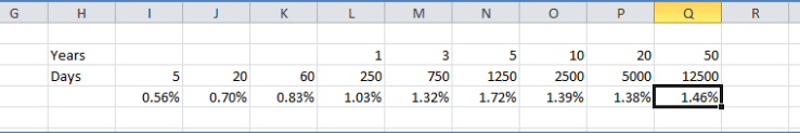
To find the average ATR overthese periods take the following steps:

·Select cell I4and type “=average(F2:F6)”.Press Enter.

·Select cell J4and type “=average(F2:F21)”.Press Enter.

·Select cell K4and type “=average(F2:F61)”.Press Enter.

·Select cell L4and type “=average(F2:F251)”.Press Enter.

·Select cell M4and type “=average(F2:F751)”.Press Enter.

·Select cell N4and type “=average(F2:F1251)”.Press Enter.

·Select cell O4and type “=average(F2:F2501)”.Press Enter.

·Select cell P4and type “=average(F2:F5001)”.Press Enter.

·Select cell Q4and type “=average(F2:F12501)”.Press Enter.

·Select cells I4 to Q4 and right-click within the selection and click Format Cells. Change the categoryto Percentageand press OK to express these values aspercentages

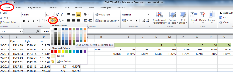
To finish the spreadsheet off, we can tidy up this table by adding some colour and borders:

·Select cells H2:Q2 and change the cell background colour to a light green by displaying the Home tab and navigating to Theme colours. 

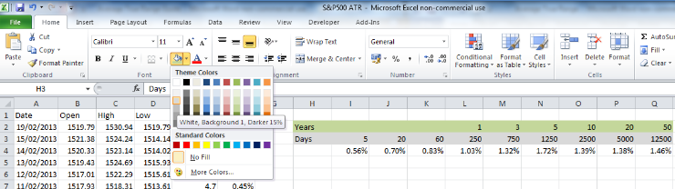
·Select cells H3:Q3 and change the colour of the cells to a light grey.

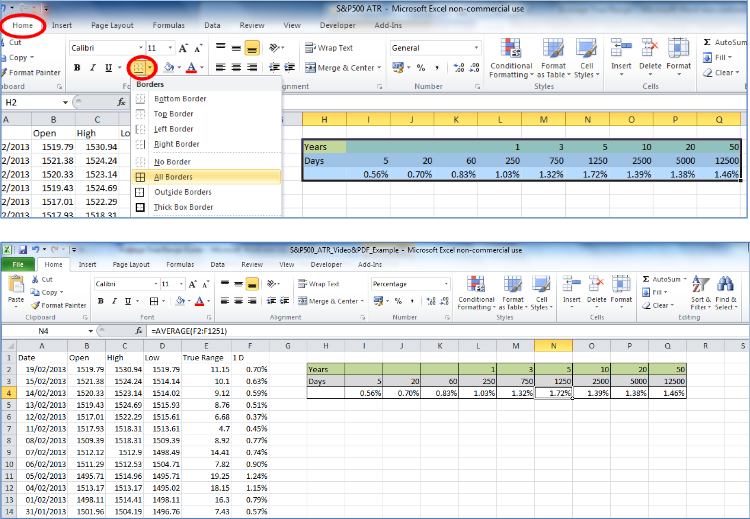
·Finally, add borders to this table by selecting cells H2:Q5 and navigating to HomeBordersAll Borders.

A note on updating your spreadsheet

If you want to keep on top of your rolling ATRs, the easiest way to do so would be to rearrange the data to show the earliest date at the top of the sheet, down to the latest date at the bottom. You can do this by applying a filter to the date column (a similar method is shown in the Returns Distribution Example), and sorting the columns from oldest to newest. Then you can manually add in the data at the bottom of the spreadsheet and update the relevantcell formulas (in cells F12872 and I4:Q4).

Summary

In this guide we calculated the one-day rolling Average True Range of the S&P500 over the last 50 years. This gives us an idea of the changes in volatility of the asset. We then calculated the average one-day ATRs over different time horizons. We can see thatover the last 50 years there has been a general tendency towards less and less daily volatility. This reiterates the fact that day trading opportunities are typically minimal, and we must wait for periods of higher volatility to take advantage of day trading. Most of the time, we require longer periods of time to see enough price movement to make our trades worthwhile. Volatility indicators like ATR help us identify when we adopt a portfolio management style of investing and when we switch to shorter term investing horizons, such as day trading strategies.