Ambiguous Wave Counts
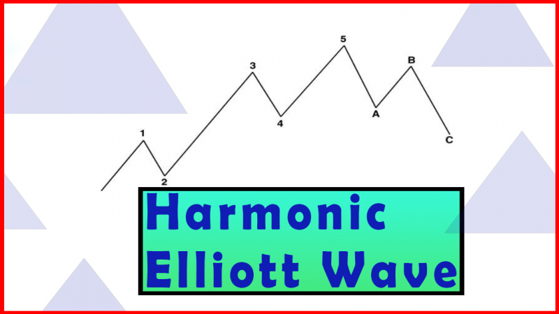
Harmonic Elliott Wave, Expanded Flat, Wave Structures, Bearish structure
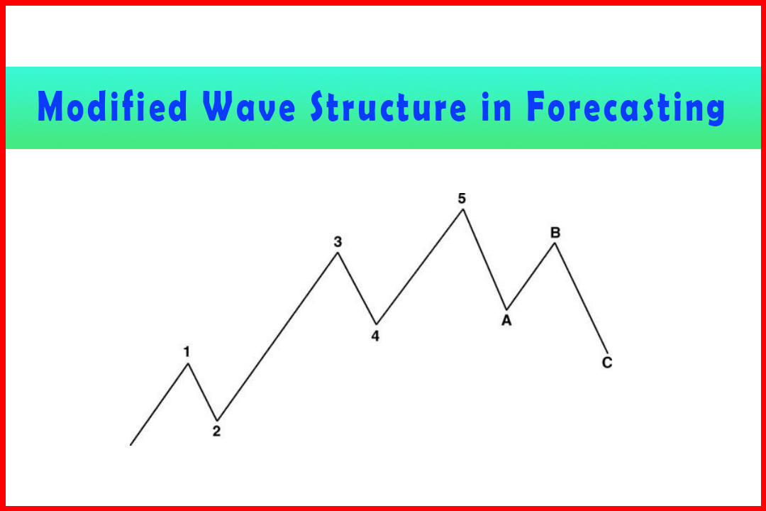
Course: [ Harmonic Elliott Wave : Chapter 5: Modified Wave Structure in Forecasting ]
Elliott Wave | Forex | Fibonacci |
It is easy to sit and write about forecasting, providing examples that hold perfect wave relationships that give the impression that all your problems are solved.
Ambiguous Wave Counts
It
is easy to sit and write about forecasting, providing examples that hold
perfect wave relationships that give the impression that all your problems are
solved. I have always taken the view that if a forecasting technique is easy
then everyone will learn the process with the idea that it will be a
self-fulfilling prophesy. Very clearly this is not the case, since if everyone
knows what the market is going to do there'll be the contrarian with
large funds to push around to hammer stop losses. As much as Harmonic Elliott
Wave is a fabulous tool, there are still numerous barriers to overcome,
confusing wave development that seems to lack any relationships, and
difficulties in identifying Wave (i) and Wave (ii) in particularly erratic
beginnings to a new wave.
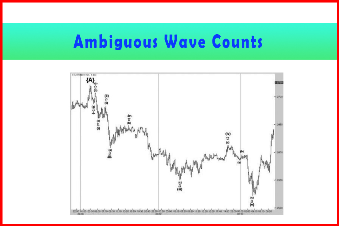
Not
all wave counts are obvious, and on occasion, because of the natural order of
Fibonacci ratios in particular, the wave relationships become ambiguous. Figure
5.22 is an example of a recent wave development in EURUSD.
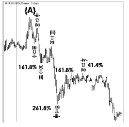
Figure 5.22 How Ratios can have Multiple Potential Relationships
Figure
5.22 is the five-minute chart of EURUSD. This correction occurred within a
rally from the June 2010 low at 1.1877, and is actually still in development at
the time of writing. I judged this to be a correction, which is yet to be
confirmed, but the rally has developed quite well within the general
expectation of this being a large Wave (IV) correction.
The
1.2722 high labeled Wave {A} was anticipated as being the Wave {A} of Wave
{III} of Wave (C) of the entire Wave (IV). The prior Wave {II} had been very
brief and shallow, exceptionally so. This raised the risk that we may see a
deep Wave {B}.
As
this Wave {B} commenced there was no way of knowing whether this would be a
simple ABC decline, a Double Zigzag, Triple Three, or possibly even a more
complex correction. Thus the initial stages of the decline were more about
judging what structure may develop. This was complicated by the fact that there
were multiple retracement ratios with a minimum of 50%:
50.0%
= 1.2518
58.6%
= 1.2482
61.8%
= 1.2469
66.7%
= 1.2449
The
first move lower from the 1.2722 peak certainly had more of a look of a
five-wave move and was labeled Wave (a). This was followed by a pullback in
Wave (b) and a decline logically in Wave (c) at 1.2661. This represented a
161.8% projection.
This
was followed by a shallow correction in Wave (x) and sharp decline to 1.2608,
which was then labeled as a second Wave (a). The appearance therefore was that
the correction was developing in a multiple ABC move. However, an interesting
development was that 1.2608 was just three points below the 261.8% projection
of Wave (a). Consideration should be given to the possibility that Wave (a)
should have been labeled Wave -i-and thus we had seen a 261.8% projection in
Wave -iii-. To verify this, the wave relationships between the decline from the
labeled Wave (x) high to the second Wave (a) should be a common extension ratio
of the decline from the labeled Wave (b) to the first Wave (c). In fact, this
turned out to be 161.8% also . . .
This
opens an ambiguous interpretation. Either the multiple ABC decline will work
through, or perhaps this was part of a five-wave decline in Wave (a) to be
followed by a retracement in Wave (b) and final decline in Wave (c) as a large
Zigzag. Given the potential for this to be a deep Wave {B}, it certainly had
reasonable grounds for consideration.
The
next measurement to take to try to clarify which structure was developing was
to look for between a 41.4% and 50% retracement in what could be Wave (b) or
Wave -iv-. The possible Wave -ii-had retraced around 61.8% and this tended to
imply a greater chance of a 41.4% retracement. It met that perfectly at 1.2649.
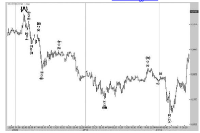
Let's
just recap what has occurred until this point.
Figure
5.23 displays the initial decline with ratios displayed. Clearly there are two
possible interpretations but with differing expectations. If the 1.2649 high
was a Wave (b) then a five-wave decline in Wave (c) will be expected; if this
is a Wave -v-decline then we must expect a three-wave decline and with
projection ratios calculated from the distance from the 1.2722 high to the
1.2608 low extended from 1.2649. These would be:
61.8%
= 1.2579
66.7%
= 1.2573
76.4%
= 1.2562
85.6%
= 1.2552
Figure 5.23 Reviewing the Wave Relationships
Therefore
there is a need to observe how the beginning of the decline develops to judge
from the structure whether it develops in three waves or five. At the end of
the decline price stalled at 1.2550, just two points below the 85.6%
projection.
Figure
5.24 displays the decline from 1.2649 appeared more to be like a five- wave
move which swayed the wave count in favor of a Triple Three, with this being
the second Wave (c) that had stalled 32 points above the 50% retracement in
Wave {B} at 1.2518. This would allow a further ABC decline that could stretch
to 1.2518 or even perhaps one of the deeper Wave {B} retracement levels.
Figure 5.24
Reviewing the Wave Relationships
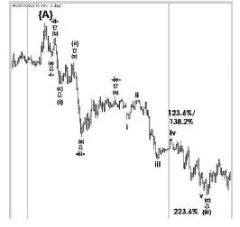
However,
there was a further complication. Now that the decline has come in two sets of
ABC moves this will mean the 1.2661 low may well be a Wave (i), which in turn
could imply a larger ABC decline with this being Wave A. The first Wave (c) was
161.8% of Wave (a). The second Wave (c) was between 123.6% and 138.2% and also
represented a 223.6% extension of the Wave (i).
Once
again, verification of the possibility of a Wave (iv) is required. Wave (ii)
had retraced close to 38.2% and therefore the Wave (iv) should be around 50%.
In fact it stalled at 1.2613, which was just short of 50% but could still
provide a projection in Wave (v), the common projections being:
61.8%
= 1.2507
66.7%
= 1.2498
76.4%
= 1.2482
Refer
back to Figure 5.22. The final low was at 1.2522, which was four points above
the 50% retracement level in Wave {B} and represented between a 50% and 58.6%
projection in Wave (v). Wave (c) was a 276.4% extension of Wave (a).
At
this point I forecast a recovery, and probably quite a deep one. However, there
was still an ambiguity. This was after all a decline of three sets of ABC
structures, and at the 50% retracement in Wave {B} could represent a completed
correction. The alternative was that given the reasonably good wave
relationships this could also be Wave A of a larger ABC decline that would see
a deep Wave B and then Wave C decline to a level closer to one of the deep Wave
{B} retracement levels.
In
fact, price maintained the recovery to new highs to confirm the 1.2522 low as
Wave {B}, and thus a rally in Wave {C} of Wave {III} was underway. There is a
further validation to be made here. This was assumed to be a Wave {iii} and therefore
there would be projections in Wave {III}, and these will need to match with a
valid projection in Wave {C}.
Harmonic Elliott Wave : Chapter 5: Modified Wave Structure in Forecasting : Tag: Elliott Wave, Forex, Fibonacci : Harmonic Elliott Wave, Expanded Flat, Wave Structures, Bearish structure - Ambiguous Wave Counts
Elliott Wave | Forex | Fibonacci |