Putting it all Together - Option Trading

Putting it all Together

Now that you understand about fair value along with the fact that volatility tends to move sideways, let’s see if we can use this new knowledge to help us check the value of an option.

Let’s go back to the VIP trade we discussed at the beginning of the chapter. To make the example easier to follow, let’s just pick one of the call options.

Since most option traders are tempted to buy the out-of-the-money strike, we will assume that we are interested in buying the $33,375 call.

Figure 1 shows that the $33,375 call was priced at $2.50 on December 16. But we also said that there can be significant differences between an option’s price and its value. Before we buy this (or any) option, we need to check the value by checking the past volatility of the underlying stock. Once we get a feel for how the past volatilities have behaved then we can gauge how much we should be willing to pay for the option.

By checking the historical volatility, we are gaining an idea of the possible payouts from the option. In other words, if VIP closes at $34,375 at expiration, that call is worth $1. If the stock closes at $35,375 it is worth $2 and so on. How likely is it that the call is worth either of these values? How likely is it that it’s worth more? To answer that, we need to know the standard deviation of the bell curve representing the stock price changes and that’s exactly what the past volatilities show us.

One of the simplest ways to check the past volatility is to view a long-term chart, perhaps one year or more, of the volatility on the underlying stock. Be­cause we are trying to determine the value of the $33,375 call, it is usually best to match the expiration with the moving average. For example, the $33,375 call expires in about 30 days so we should use a 30-day moving average for the historic volatility. Figure 8 shows a one-year chart of the 30-day moving aver­ages for the volatility of VIP stock:

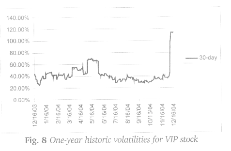
If you look at Figure 8, you will see that the average has just moved between a low of 30% and high of about 70% with the exception of the spike at the end of the chart approaching the 120% level.

Now we have a decision to make. Which volatility level will be correct for the next thirty days until expiration of the calls? While we will never know the correct answer until after the fact, we do know the long run history has been between low of 30% and a high of 70% so our estimate should probably lie in this region. Figure 8, however, shows that the current level of volatility is near 120%. If we use this volatility to price the option, we will probably be fighting a downward pull on the option’s price, as the volatility will most likely fall back to the average. Remember, the price of an option is directly tied to the volatility. If the volatility is high then so is the price. But if we are expecting volatility to fall, then the price of the option will fall as well if our expectations are correct.

Prior to the large spike in Figure 8, the 30-day volatility had just crossed the 40% so that might be an estimate for future volatility over the next 30 days. Although 40% is one estimate, it is not the only one we could use. Remember that volatility is the only true unknown in the Black-Scholes Model and now you see why - volatility does not stay constant. However, most option traders would agree that the future volatility estimate should be fairly representative of the moves we observe in the chart. If we were to ask many option traders for their opinion on future volatility, we might obtain estimates in the shaded area of Figure 9:

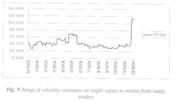
Traders with a strong bullish conviction may be willing to buy the option with a volatility level at the high end of the shaded area, say 60%. Traders less convinced of a large price move in the stock may only be willing to buy the option at the lower end of around 40%. But very few traders should be willing to pay the current level of 120% since that is a very rare volatility level. This shows why it is not a good idea to rely on software that compares a single point (such as the 30-day average) to the current price. Under this system, the soft­ware would tell you that an option priced at 120% volatility’ is fairly priced even though that’s far from true based on historical standards.

Let’s assume we split the difference between the 40% and 60% levels and use 50% for our future volatility estimate. What does the Black-Scholes Model say about the value of this option?

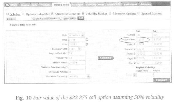
We know the current stock price is $31.41, we’re interested in buying the $33,375 strike, there are 39 days until expiration, no dividends are paid on the stock over the life of the option, and we just decided to use 50% as a future estimate of volatility. (Remember, this calculator automatically finds the risk- free interest rate for you.) Figure 10 shows that the fair value of a call option with these inputs is only about $1.30:

There is clearly a discrepancy between what we think the call is worth when compared to the $2.50 market price. In other words, the $2.50 market price of the option is far greater than the $1.30 value to us.

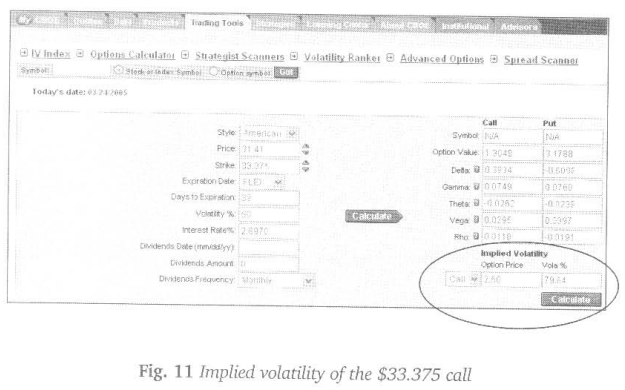
We said earlier that there are two ways we can view a bet and now it’s time to take a look at the second way. Let’s assume that the market is correct and that the $2.50 asking price is a fair value for this bet. Which volatility must the market use to come up with a price of $2.50? We can find out by simply entering the $2.50 asking price into the “implied volatility” section in the lower right hand corner of the calculator, which is circled in Figure 11. (Make sure you also select “call” from the drop down menu.) After we lilt the “calculate” bar in the same circle, the calculator shows that the market is using a volatility estimate of nearly 80% (79.64%).

The implied volatility shows us the volatility level that must be used in order to make the current market price true. The market does not agree with our 50% estimate and is, instead, using a volatility of nearly 80%. If you type 79.64 into the “volatility %” box on the left hand side of the calculator, the price of the call would show $2.50. Just as with our coin toss example, the market does not need to specifically think that the future volatility is 80%. The mere fact that traders are willing to pay $2.50 for the call implies that they are using 80% as an estimate of future volatility. It is for this reason that the 80% figure is called the implied volatility. What likely caused this high level of volatility is the fact that traders continued to buy up these call options without consulting a pricing model.

Now, as option traders, we have a decision to make: Does 80% seem like a reasonable estimate of future volatility? After checking the volatility over the past year, we find that it does not seem to be in line with any of the volatilities we’ve seen in the past with the exception of the recent spike. This does not mean that it’s impossible to make money with this option if we were to pay $2.50. Instead, it shows that the odds appear to be stacked very much against us. It is a trade we’re better off avoiding. In our opinion, this appears to be a losing proposition if we were to make this exact trade hundreds of times.

Why does $2.50 appear to be an unfair price? If you pay $2.50 for this option, there is a very good chance that volatility will revert to the average - dragging down the option’s price with it. And that is exacdy what happened with the VIP calls in Figure 1.

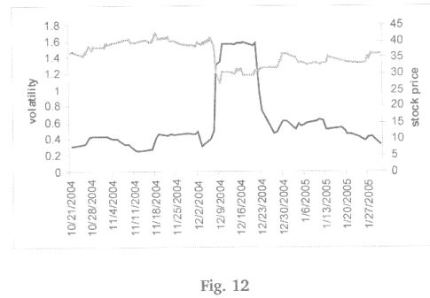
Figure 12 shows an overlay of the stock’s price (shaded line) and the 10- day historical volatility (bold line). You can see that the stock’s price did rise after December 16 but that volatility also fell right back to the average as we expected. The net result between these two forces was an overall loss. It was the falling volatility that was the culprit of the call losses.